Common metrics to evaluate recommendation systems
Are your evaluation metrics top-heavy?

The offline evaluation of recommendation systems is one of the most critical criteria for comparing different algorithms and selecting the best performing model to deploy in production. In this blog, we will take a look at some of the common metrics used to evaluate recommendation systems. Most of these metrics are defined in On Sampled Metrics for Item Recommendation paper where the authors discuss the properties of these metrics when evaluation data is sampled. This blog will lay the foundation for discussing the interesting ideas mentioned in the paper, by taking a look at what are some common metrics for item recommendation and how do these useful metrics possess a top-heavy property.
First, we start off with a discussion on what are recommendation systems and how to define a generic metric to evaluate a recommendation system.
What is a Recommendation System?
The high-level idea behind an item recommendation system is to rank a large catalog of items and show only top most relevant items to the user. Usually, recommendation systems use user-item interaction data, e.g. the number of times a product was viewed / purchased on Amazon by a particular user, the number of times a movie / series was watched on Netflix by a viewer, etc. In some cases, recommendation systems can also leverage additional data such as social network data of users or knowledge graph data of catalog of items. Based on this information, recommendation systems build a mathematical model that can accurately predict the items that a particular user might be interested in. This is a challenging task as the catalog of items is large: “tens of thousands in academic studies and often many millions in industrial applications”, and only a top few of those items can be shown to the user.
How to Evaluate?
As users get to see only top-k recommended items, the recommender systems are usually evaluated using top-heavy metrics that assign higher scores to models which rank most of the relevant items in top-k. A top-heavy property of a metric implies that the metric gives higher scores to an algorithm which performs very well on top few items and discards (or gives lower importance to) the scores for other items.
Some Notations
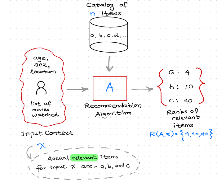
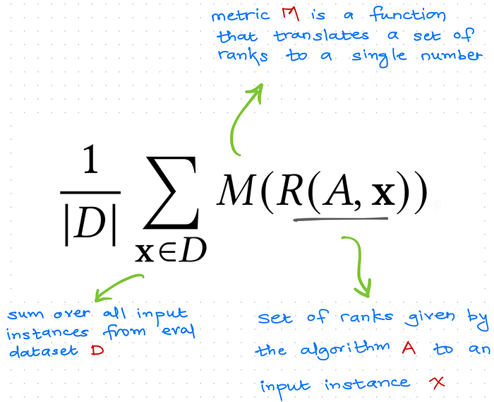
Let there be n items in the catalog. For a given input instance x (where an instance can be user or item or a context query), a recommendation algorithm A outputs a ranked list of n items. To evaluate this ranked list of items, the positions of relevant items, denoted by R(A, x), in the ranked list are considered. Here, R(A, x) would be a subset of {1, 2, …, n} and contains the ranks of actual relevant items given by the algorithm A for an input x. For example, R(A, x) = {3, 5} means that for input x, there were two relevant items in the catalog, and recommender system A ranked these items at positions 3 and 5 respectively. Then we use a metric M that translates the ranks of relevant items into a single number measuring the quality of the ranking. This process is repeated for a set of input instances from an evaluation dataset D = {x1, x2, … } and the average metric is reported as the performance of A on evaluation dataset:
Example
Consider an example of recommendation system for Netflix users. The input instance here could be a context comprising information of a particular user (e.g. age, gender, location, etc.) and his / her interactions with the items (e.g. recently watched movies/series etc.). For this input, let’s assume that there are 3 items on Netflix that are relevant to the given context. Then the output would be a set of ranks given to those 3 items by the recommendation system (say, {5, 10, 20}). We would then use a metric to map these ranks to a single number indicating how good or bad the ranks of the relevant items were. Finally, we repeat this for all contexts in the evaluation dataset (e.g. context inputs generated using some users and their historical interactions) and calculate the average metric as the performance of the recommendation system.
Metrics
In this section, we take a look at some of the common metrics that can be used for evaluating recommendation systems.
These metrics are mentioned in On Sampled Metrics for Item Recommendation.
Area Under ROC Curve (AUC)
AUC measures the likelihood that a random relevant item is ranked higher than a random irrelevant item. Higher the likelihood of this happening implies a higher AUC score meaning a better recommendation system. We calculate this likelihood empirically based on the ranks given by the algorithm to all items — out of all possible pairs of type (relevant-item, non-relevant-item), AUC is a proportion of pairs where relevant-item was ranked higher than the irrelevant item from that pair.

Precision @ K
Precision is an indicator of the efficiency of a supervised machine learning model. If one model gets all the relevant items by recommending fewer items than another model, it has a higher precision. For item recommendation models, precision at k measures the fraction of all relevant items among top-k recommended items.

Recall @ K
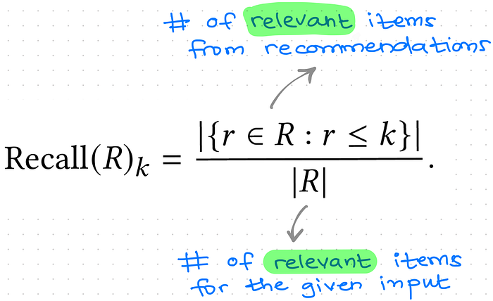
Recall is an indicator of the effectiveness of a supervised machine learning model. The model which correctly identifies more of the positive instances gets a higher recall value. In case of recommendations, the recall at k is measured as the fraction of all relevant items that were recovered in top k recommendations.
Average Precision @ K
measures the precision at all ranks that hold a relevant item.
Consider a scenario where we have following top-5 recommendations from two recommender systems A and B for the same input.

Here, both the recommender systems were able to capture 2 relevant items (s and t) in the top-5 recommendations. Thus both would get the same precision@5 score. But, clearly the model A is better than model B as it recommended the relevant items at position 1 and 2, whereas model B recommended them at position 4 and 5. This is exactly the problem the average precision metric tries to solve. It essentially calculates the precision at every location 1 through k where we have a relevant item.

Normalized discounted cumulative gain (NDCG) @ K
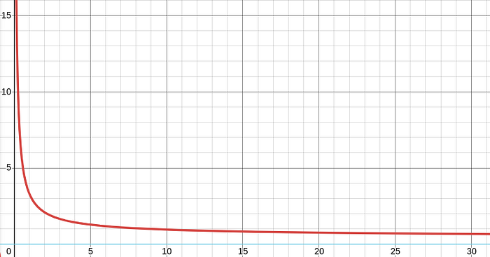
NDCG measures the overall reward at all positions that hold a relevant item. The reward is an inverse log of the position (i.e. higher ranks for relevant items would lead to better reward, as desired).

The following graph shows inverse log at different locations. The inverse log has a top-heavy property and therefore it’s suitable for evaluating recommendation systems.
Other metrics
There are other metrics that are not discussed in the paper. E.g. Mean Reciprocal Rank (MRR) calculates an average of reciprocal of ranks given to the relevant items. So if the relevant items are ranked higher, the reciprocal of the ranks would be lower leading to a lower metric score, as desired. Essentially, the idea behind evaluating a recommendation system is to make use of ranks given to the relevant items and translate into a single number indicating how good or bad the ranks are (remember that ideally we would want to have the ranks as 1 for all the relevant items).
Comparison of Metrics
For simplicity, let’s assume that there is only 1 relevant item in the catalog for a given input instance (e.g. only 1 relevant movie on Netflix for a given user and his / her historical behavior). In this case, the metrics discussed above would map the rank of this relevant item given by the recommendation system to a single number. The following plots show the metric for different ranks of the relevant item.

Here, the catalog contains n = 10,000 items. The rank r given by the algorithm for the relevant item for a given input query could be any number between 1 and 10,000 (i.e. r belongs to set 1 to 10,000). The plot above indicates the value given by each of the metrics for every possible rank r of the relevant item. The plot below zooms on the scenarios when the relevant item is ranked in top 100 items.
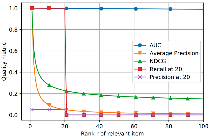
All metrics besides AUC are top heavy and almost completely ignore the tail. i.e. AUC changes linearly with the rank of the relevant item (e.g. reward for pushing the rank from 1000 to 999 is the same as reward for pushing the rank from 10 to 9). This is undesirable as users get to look at very few top ranked items. So we want to use metrics that reward 10-to-9 jumps much higher than say 1000-to-999 ones. Thus, AUC does not serve as a good metric for recommendation systems, and top-heavy metrics are correct choices to evaluate recommendation systems.
Upcoming topic
Hopefully, we all now have a high-level idea about how recommendation systems are evaluated. In the next blog post (yet to be published), we will discuss how these metrics behave when we apply sampling during evaluation. This sampling process leads to interesting mistakes when selecting the best recommendation system based on the sample metrics calculated during offline evaluation, so stay tuned!
